Index:
1. Software Introduction
2. Software Structure
3. Data Required
4. Trajectory Ensemble Receptor Model Algorithm
4.1 Conditional Probability Function (CPF)
4.2 Concentration Field Analysis (CFA)
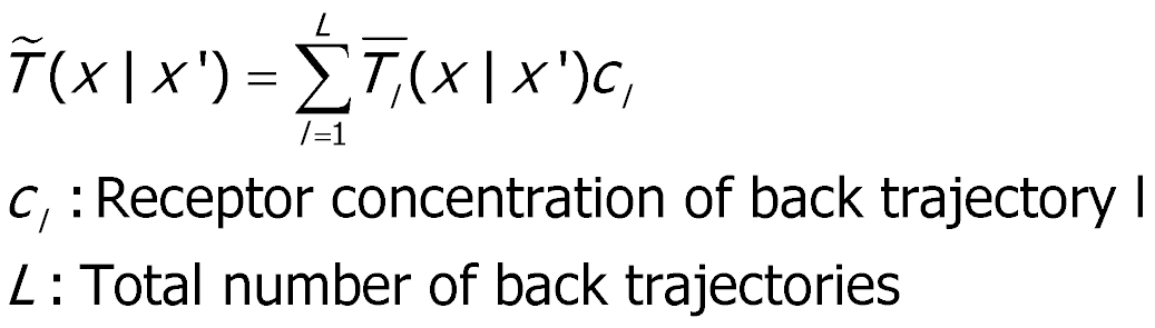
4.3 Concentration Weighted Trajectory (CWT)
4.4 Residence Time Weighted Concentration (RTWC)
4.5 Potential Source Contribution Function (PSCF) and multiple-site PSCF
4.6 Simplified Quantitative Transport Bias Analysis (SQTBA)
5. Trend Analysis Algorithm
5.1 Kendall's tau
5.2 Sen's Slope
6. GIS Function Algorithm
6.1 Grid Smoothing
6.2 Grid Peak Identification
6.3 Grid Weight
7. Acknowledgement
View User's Guide and Examples.pdf
1. Software Introduction:
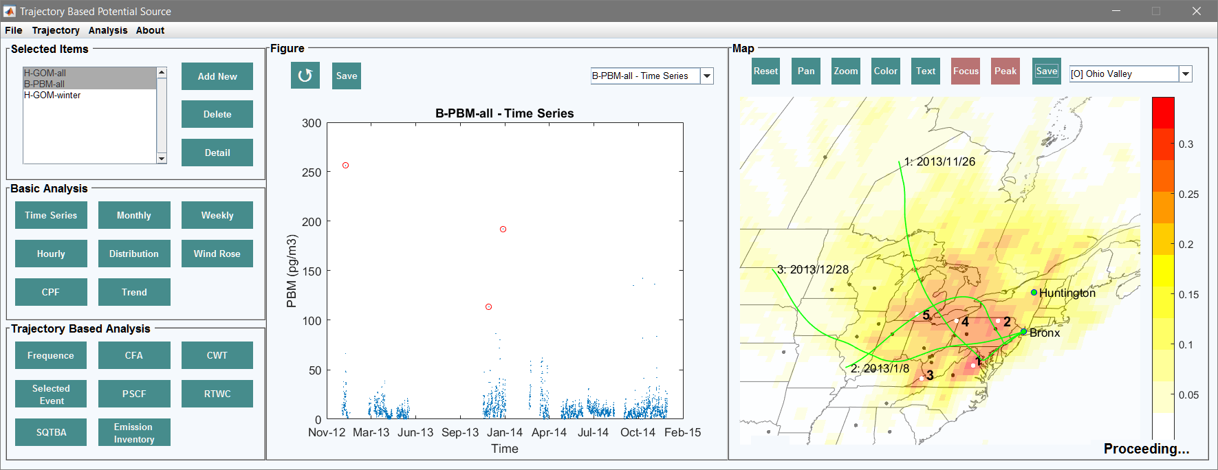
TraPSA (Trajectory-based Potential Source Apportionment) software is a graphical air pollution source analysis tool based on air pollutant measurements and a state-of-art air mass back trajectories model HYSPLIT-4. TraPSA provides researchers and students an integrated, user-friendly platform for air pollutant database development and management, pollutant pattern and trend analysis, and potential source identification, by applying, comparing and exploring current popular trajectory ensemble receptor models.
Main Interface of TraPSA A database of pollutant monitoring site data can be established in TraPSA. The smart back-trajectory method in TraPSA helps users easily set up, calculate, and import trajectory data. TraPSA includes current popular algorithms for trajectory ensemble receptor models including Conditional Probability Function (CPF), Concentration Field Analysis (CFA), Concentration Weighted Trajectory (CWT), Residence Time Weighted Concentration (RTWC), Potential Source Contribution Function (PSCF), and Simplified Quantitative Transport Bias Analysis (SQTBA). TraPSA provides users sufficient GIS editing functions for mapping air pollutant source apportionment. In addition, GIS data files (ESRI shape file and Geo TIFF file) can be imported or exported by TraPSA allowing further research or editing by GIS software.
TraPSA was developed as an extension package of HYSPLIT_4 software and can be linked to local HYSPLIT_4 installations on the computer. However, TraPSA can also be used without installation of the full HYSPLIT_4 software suite because TraPSA software includes an unregistered version of the HYSPLIT_4 trajectory model executable. However, it is strongly recommended that users register and install the most current version of HYSPLIT software in order to generate the most accurate trajectories.
TraPSA was programed in MATLAB 2015b. It is only executable on Windows OS platforms and a 1920 X 1080 screen resolution is recommended. MATLAB Runtime is required to run TraPSA so that the full version of MATLAB is not necessary. MATLAB runtime will automatically be downloaded if it hasn’t already been installed on the computer.
Go Top
2. Software Structure:
The structure of TraPSA is shown in the following figure. Pollutant measurement data, meteorological data and ESRI shapefile of related geographic region (grey blocks) are required. An air pollutant monitoring site database should be established with site information and pollutant measurement data. Trajectory endpoints will be generated based on pollutant measurement date using meteorological data and HYSPLIT model. As an optional data-input, trajectory endpoints can be imported into the database if the files were previously generated by HYSPLIT_4.
Structure of TraPSA After program execution, pollutant data and corresponding trajectory endpoints can be extracted from the database and used for analysis. TraPSA contains modules to compute pollutant pattern analysis, trend analysis, and trajectory ensemble receptor models (including CPF, CFA, CWT, RTWC, PSCF, and SQTBA) for potential source location identification. An ESRI shapefile of the geographic region is required to correctly display the results of the trajectory ensemble receptor models. Any figures generated by TPBS can be exported including their numerical data. Trajectory endpoints and the map raster can be exported in GIS data formats (ESRI shape file and Geo TIFF file) if further analysis and/or editing is necessary in other GIS software.
Go Top

3. Data Required:
Meteorological data (wind feild data) is required by TraPSA for generating HYSPLIT trajectories. Various meteorological data formats are available as long as they are recognizable by HYSPLIT_4, although the HYSPLIT_4 suite contains numerous converters that users can use to convert data into HYSPLIT format. Typically, the Eta Data Assimilation System (EDAS) with the 40 km resolution data and North American Regional Reanalysis (NARR) data are used for North American locations. The Global Data Assimilation System (GDAS) and the NCEP/NCAR Reanalysis Archive have been used for sites in Europe and Asia. In addition, NOAA ARL maintains an archive of meteorological datasets called "Ready" in HYSPLIT format that can be used to drive the HYSPLIT trajectory model (as well as other HYSPLIT executables).
ESRI shapefiles are required to display maps in TraPSA. Two GIS data formats, ESRI shapefile (‘.shp’, ‘.dbf’ and ‘.shx’) and GeoTIFF file (‘.tif’) are available for used by TraPSA. Shapefiles of related regions should be downloaded before analysis. Note that it will take a longer time to display the shapefiles with more geographic information.
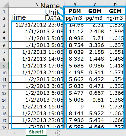
Pollutants measurement data are required for receptor models. The data file format can be ‘.cvs’, ‘xlsx’ or ‘.xls’. The data should include species names, units, collection date and concentration and organized as shown in the following figure. Note that collection date format is flexible as long as it can be identified by TraPSA, but must include year, month, day and hour information. TraPSA will handle the date format, missing data and replicate data automatically.
Input Pollutant Data File Format
4. Trajectory Ensemble Receptor Model Algorithm:
TraPSA includes current popular algorithms of trajectory ensemble receptor models including Conditional Probability Function (CPF), Concentration Field Analysis (CFA), Concentration Weighted Trajectory (CWT), Potential Source Contribution Function (PSCF), Residence Time Weighted Concentration (RTWC), and Simplified Quantitative Transport Bias Analysis (SQTBA). Each model is described in more detail below. Please note that CPF, CFA, CWT, PSCF are inherently single site approaches (PSCF has a particular multiple site approach) whereas RTWC and SQTBA are designed as multiple site models though all these models (except CPF) could be applied either in single or multiple sites in TraPSA software.
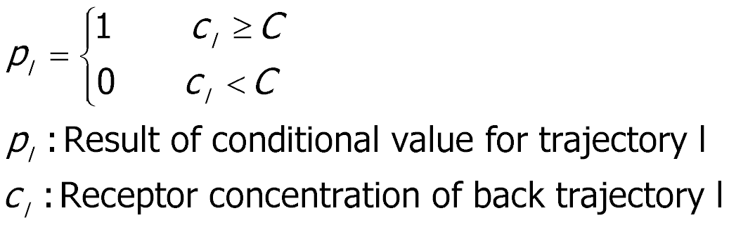
4.1 Conditional Probability Function (CPF)
CPF determines the probability of a wind direction to be associated with specific pollutant levels and can be useful for determining local source directions. A criterion value C (which is adjustable in TraPSA) representing high concentration events is arbitrarily set (usually 75%~90% of the highest concentration). The CPF value for different wind directions is calculated as:
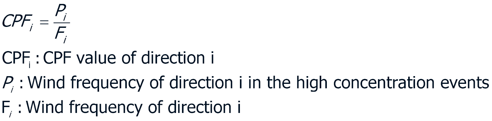
Note that the wind direction has a large uncertainty for low speeds (typically [5 km/h] although the parameter can be manually set). Therefore, these data should be discarded. Also note that the wind speed and direction, which are generated by HYSPLIT4, will probably change with the trajectory starting height used.
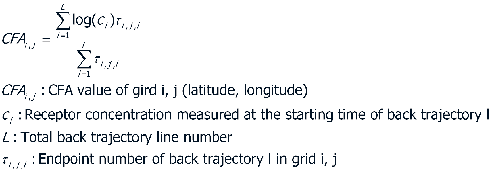
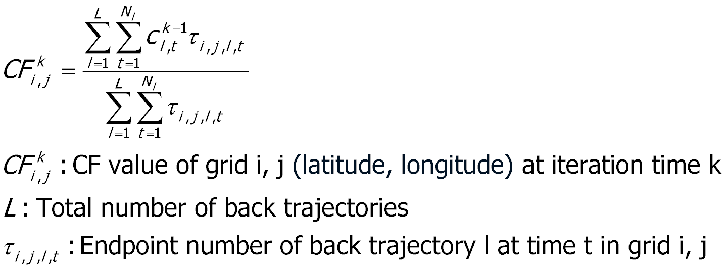
4.2 Concentration Field Analysis (CFA)
The CFA model determines air pollutant source locations by combining concentration measurements with back trajectories. For this method, the whole geographic region is divided into an array of grid cells defined by the cell indices i and j. Backtrajectories (presented by l) will be generated starting at concentration measurement time at receptor site. Trajectory endpoints in grid cells (presented by τ) will be counted after back-trajectory calculations. If a trajectory endpoint lies in the grid cell, the trajectory is assumed to collect and transport the material emitted in this cell along the trajectory to the receptor site. The CFA values then can be calculated as shown below so that grid cell with larger CFA value implies the higher contribution of pollutant to the receptor site:
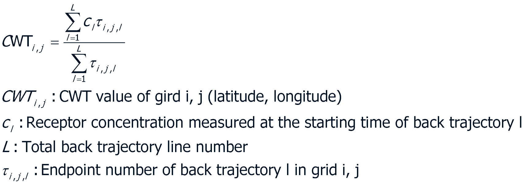
4.3 Concentration Weighted Trajectory (CWT)
The concentration field values of the grids that a trajectory passes through with a concentration close to 0 will significantly reduce their CFA due to the logarithmic calculations used in CFA. The CWT model is a modification of CFA using a linear calculation, which is more robust to low pollutant measurements. The CWT values are calculated as follows:
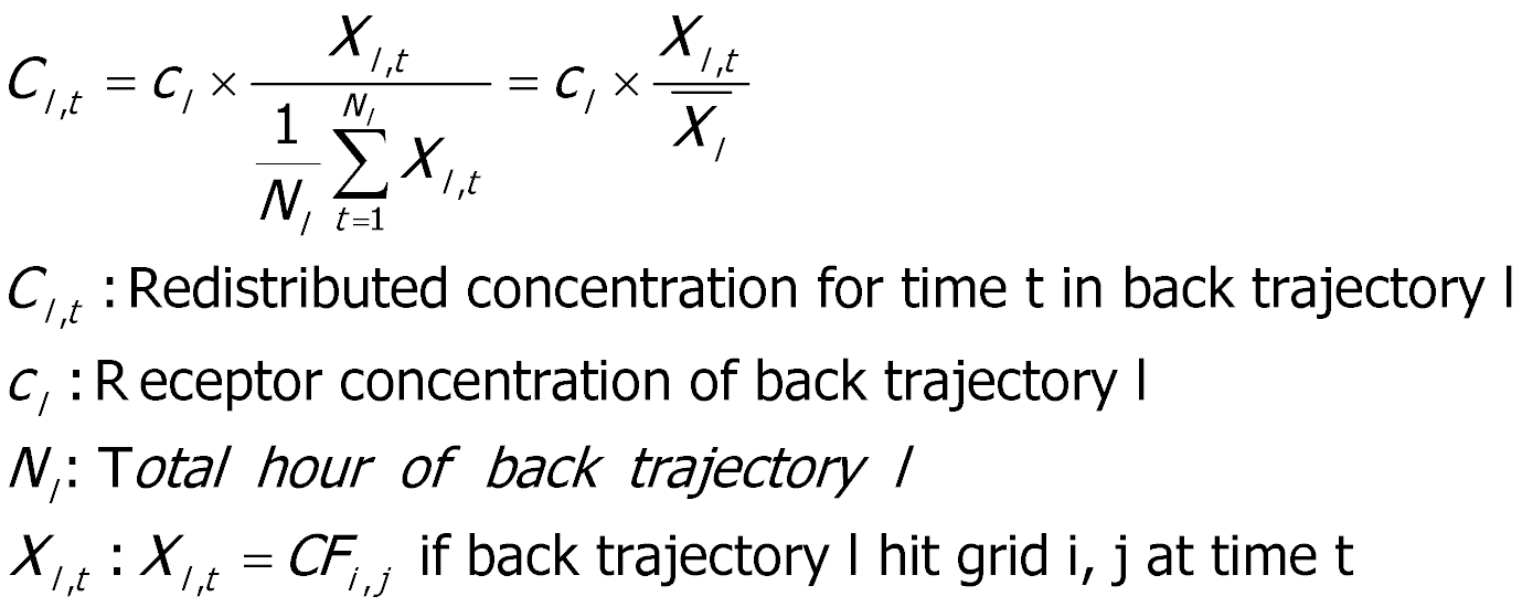
4.4 Residence Time Weighted Concentration (RTWC)In order to distinguish a large source from a moderate source, the RTWC model can be used for calculate a grid concentration field. The rational for the redistribution used in the RTWC approach is that no major pollutant sources are located along a “clean” trajectory (i.e. one with a very low concentration at the receptor site). The “polluted” trajectory (i.e. one with a high concentration at the receptor site) must have been influenced by sources along its path through which no “clean” trajectories pass. Also RTWC can be applied into multiple sites since a trajectory going to one monitoring site cannot typically go to another and thus, it helps clean up trailing effects.
The initial field can be calculated by the CWT or CFA model and the redistributed concentrations for every trajectory can be calculated:
Then concentration field is iterated until the average difference between the concentration fields of two successive iterations is below a criterion value (typically 0.5%):
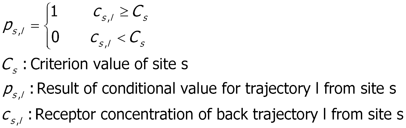
4.5 Potential Source Contribution Function (PSCF) and multiple-site PSCF
The PSCF model calculates conditional probabilities (if the value is close to 1 means the trajectories cross the grid cell effectively transport the emitted contaminant to the receptor site) to identify the source contribution of each grid to receptor site. The contribution function is determined by a criterion value C (the parameter is adjustable in TraPSA), which is arbitrarily set (usually 50%~90% of the highest concentration). The contribution value of the endpoint on a back trajectory with receptor concentration larger than C is 1, otherwise the contribution value is 0:
Then PSCF values are calculated as follow:
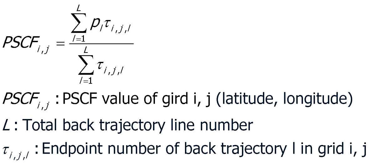
The PSCF model can't be directly applied into multi-site analysis as a fixed criterion value is used. The multi-site PSCF model is defined as:
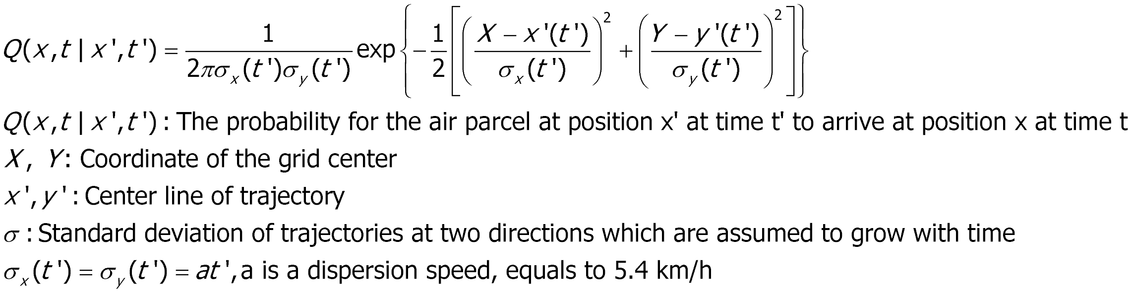
4.6 Simplified Quantitative Transport Bias Analysis (SQTBA)
The uncertainties in a trajectory pathway increase with the increasing trajectory length. These uncertainties are considered in the SQTBA model, a simplification version of QTBA. SQTBA assumes a normal distribution caused by atmospheric dispersion is approximated about the trajectory centerline with a standard deviation that increases linearly with time in the upwind direction. Thus the transition probability density function can be expressed as:
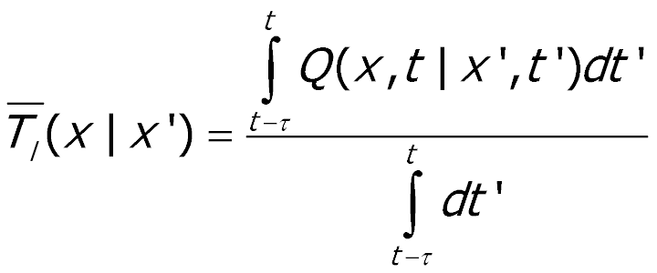
The potential mass transfer potential field for a given trajectory l, arriving at time t, is integrated over back trajectory time τ:
The concentration-weighted mass transfer potential field is calculated as:
Then final SQTBA field is obtained as follow:


5. Trend Analysis Algorithm:
Detecting and assessing temporal trends in long-term air pollutant concentrations is important for environmental studies, monitoring programs, and evaluating air pollution control policies. Trend evaluations are frequently used to determine whether it is reasonable to assume concentrations are temporally stationary (for example, to perform statistical evaluations that require stationary means) and to detect or model decreasing trends to support natural attenuation studies.
TraPSA includes Kendall's tau and Sen's slope for trend analysis.
5.1 Kendall's tau
Kendall’s tau is a non-parametric measure of correlation between two data series. It determines whether the trend is positive or negative and the strength of correlation between two data series. A negative correlation indicates that when X is increasing then Y is decreasing. It determines the difference between the probability that the observed data are in the same order versus the probability that the observed data are not in the same order. A higher absolute value of Kendall’s tau implies a stronger positive or negative correlation.
Go Top
5.2 Sen's Slope
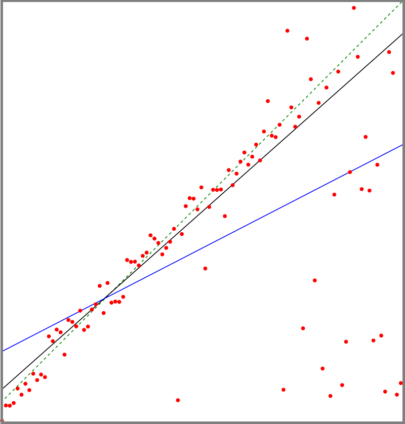
Sen’s slope is a nonparametric linear regression models, which is robust to outliers and non-normality in residuals. This method has been widely used in climate and hydrological trend analysis. Sen’s slope is defined as the median of the slopes (yi-yj)/(xi-xj) determined by all pairs of sample points in a set of two-dimensional points (xi, yi).
The Theil–Sen estimator of a set of sample points with outliers (black line) compared to the non-robust simple linear regression line for the same set (blue). The dashed green line represents the ground truth from which the samples were generated (figure source).
6. GIS Function Algorithm:
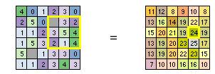
TraPSA provides a basic grid smoothing and focalization function that is calculated as shown in the following method:
6.2 Grid Peak Identification
TraPSA provides a basic grid peak identification function. One grid will be recognized as a peak grid if its value is larger than any other surrounding grids. The identified peak grids will be sorted by grid value from high to low. The number of highest peak grids is adjustable in TraPSA.
Go Top
6.3 Grid Weight
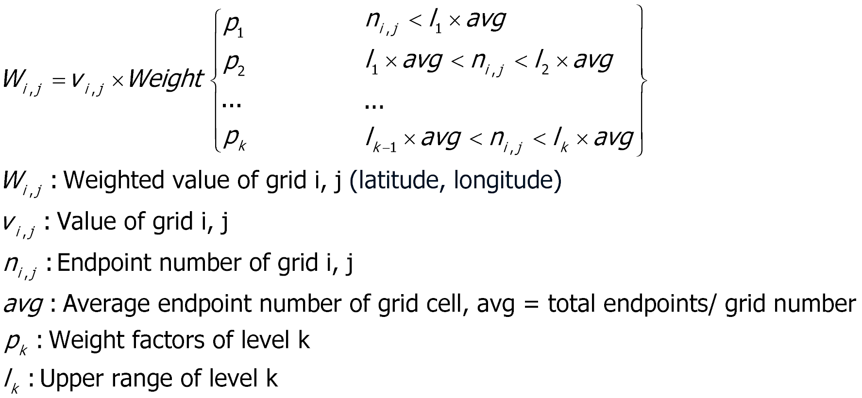
When cells are crossed by small number of trajectories, false source areas maybe identified if some of the trajectories also pass real through actual source areas; this phenomenon is called the “trailing effect”. A weighting function can be used to avoid the “trailing effect” defined as follows:
7. Acknowledgement:
Dr. Thomas M. Holsen, the Director of the Center for Air Resource Engineering & Science (CARES), Clarkson University, was the TraPSA project advisor and advised on the software structure.
Dr. Philip K. Hopke (retired), the past Director of the Institute for a Sustainable Environment (ISE), and Center for Air Resource Engineering & Science (CARES), Clarkson University, made valuable suggestions on trajectory ensemble receptor models.
Dr. Mark Cohen, NOAA Air Resources Lab, contributes to the linkage between TraPSA and HYSPLIT software.
Hao Zhou, Ph.D candidate of Institute for a Sustainable Environment (ISE), Clarkson University, did most software testing work.
CHINA SCHOLARSHIP COUNCIL, was funding the expenses of software developer in U.S.